Prof. John Rust, Hiu Man Chan
Spring, 1999
QUESTION 1 First order condition satisfied by the MLE is
![]()
Taylor series expansion around ![]() yields
yields
![]()
where ![]() is between
is between ![]() and
and ![]() .
Rearranging yields
.
Rearranging yields

For the first term, ![]() implies
implies ![]() and
and ![]() , and by LLN and
continuous mapping theorem, we have
, and by LLN and
continuous mapping theorem, we have
![]()
For the second term, by CLT for triangular arrays. (See Note below).
![]()
Finally by Slutsky theorem,
![]()
Therefore MLE is regular.
To establish this result, we need (i) ![]() int
int ![]() so
that
so
that ![]() , (ii)
, (ii) ![]() are independent, and (iii)
Lindeberg condition
are independent, and (iii)
Lindeberg condition
For all ![]()
![]()
where

in order to apply CLT for triangular array ![]() .
.
Note: The CLT needed above for the second term is not the usual sort of CLT, but a special CLT for triangular arrays.
Definition: A triangular array is a doubly
indexed sequence of random vectors ![]() where
the index i runs from
where
the index i runs from ![]() for each
N and the index N runs from
for each
N and the index N runs from ![]() . Furthermore
for each N, the sequence
. Furthermore
for each N, the sequence ![]() is
IID.
is
IID.
Note that the random vectors ![]() are a triangular array, since for each N the random variables
are a triangular array, since for each N the random variables
![]() ,
, ![]() is an IID sequence from the density
is an IID sequence from the density
![]() . It follows
that
. It follows
that ![]() ,
, ![]() is also an IID sequence, and thus the sequence
is also an IID sequence, and thus the sequence
![]() is a
triangular array of random vectors.
is a
triangular array of random vectors.
We now sketch the proof of a central limit theorem for triangular
arrays of random variables. This proof can then be extended to a
proof of the CLT for triangular arrays of random vectors via the
Cramer-Wold device, i.e. if ![]() is a triangular
array of random vectors in
is a triangular
array of random vectors in ![]() and we can show that for each non-random
vector
and we can show that for each non-random
vector ![]() that
that ![]() is a triangular array
of random variables that satisfy the CLT with asymptotic
distribution
is a triangular array
of random variables that satisfy the CLT with asymptotic
distribution ![]() where
where ![]() is a
is a ![]() covariance matrix, then we can conclude that the original sequence
covariance matrix, then we can conclude that the original sequence
![]() satisfies a (vector) CLT with asymptotic distribution
satisfies a (vector) CLT with asymptotic distribution
![]() .
.
CLT for Triangular Arrays of Random Variables
Consider a triangular array of random variables ![]() satisfying
satisfying
![]() and
and ![]() . If
. If
![]() then we have:
then we have:
![]()
Proof: (sketch) We show the moment generating function
for the normalized sum ![]() converges to the moment generating for a
converges to the moment generating for a ![]() , i.e.
, i.e.
![]() . We have
. We have
where ![]() is the moment generating function
for
is the moment generating function
for ![]() . We can do a Taylor series approximation of this
function about 0:
. We can do a Taylor series approximation of this
function about 0:
where ![]() is a point on the line segment joining
is a point on the line segment joining
![]() and 0. Note that by the
basic property of moment generating functions we
have
and 0. Note that by the
basic property of moment generating functions we
have ![]() , and
, and
![]() . Furthermore the
assumption that
. Furthermore the
assumption that ![]() implies that
implies that
![]()
Now substituting equation (2) into equation (1) we obtain
![]()
Now we use a result from calculus (which can be proved by taking logs
and appealing to L'Hôpital's rule) that if ![]() then
then ![]() .
Using this result we obtain:
.
Using this result we obtain:
Equation (3) shows that the limit of the limit of the
moment generating function of the normalized sum ![]() equals the moment generating function for
a
equals the moment generating function for
a ![]() random variable. By appealing to Bochner's
theorem (which actually requires characteristic functions, which
is simply the moment generating function evaluated at t i instead
of t, where
random variable. By appealing to Bochner's
theorem (which actually requires characteristic functions, which
is simply the moment generating function evaluated at t i instead
of t, where ![]() ), it follows that the normalized
sum
), it follows that the normalized
sum ![]() converges in distribution to a
converges in distribution to a ![]() random variable, completing the proof of the CLT for triangular arrays.
random variable, completing the proof of the CLT for triangular arrays.
QUESTION 2
Twice differentiating ![]() , we get:
, we get:
![]()
Hence,
![]()
And we know
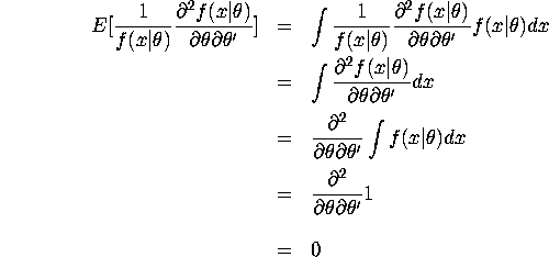
where the third equality holds by assuming that the regularity conditions
for interchanging integration and differentiation operations hold.
Therefore,
![]()
QUESTION 3
Let's assume that all the six assumptions given in your class notes hold.
To find the asymptotic distribution of the NLLS estimator, we first establish its
consistency.
Let
![]()
and
![]()
Then ![]() .
.
Now since

and the first term is independent of ![]() . Therefore
. Therefore
![]()
Under correct specification, it is clear that ![]() , so
, so ![]() . Under misspecification, the NLLS estimator converges to a point
. Under misspecification, the NLLS estimator converges to a point
![]() that gives the best mean squared approximation in the parametric family
of
that gives the best mean squared approximation in the parametric family
of ![]() to
to ![]() .
.
Next, using the fact that ![]() (in
more accurate term,
(in
more accurate term, ![]() ),
perform Taylor Series Expansion about
),
perform Taylor Series Expansion about ![]() :
:
![]()
With ![]() . Rearranging the terms, we get
. Rearranging the terms, we get
![]()
Note that the data is iid, and that
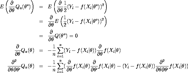
Therefore we can apply Uniform Law of Large Numbers to obtain
![]()
And by Central Limit Theorem,
![]()
As a result, by Slutsky Theorem,
![]()
Under correct specification, ![]() can be simplified since with
can be simplified since with
![]() ,
,
![]()
Therfore,
![]()
Furthermore, as ![]() are iid and independent
of
are iid and independent
of ![]() , we have
, we have

Where ![]() is the variance of
is the variance of ![]() .
.
With cancellations we finally get:

QUESTION 4
![]()
where we are instructed to believe that
![]() are IID
draws from
are IID
draws from ![]() and
and ![]() . Actually you were mislead: the errors
. Actually you were mislead: the errors
![]() are heteroscedastic, so conditional on
are heteroscedastic, so conditional on ![]() we have
we have
![]() where
where
![]() . So you will be estimating a
misspecified model, and later in Econ 551 we will discuss
test statistics which are capable of
detecting this misspecification. In the meantime your job is to calculate the
MLE's of the parameters,
. So you will be estimating a
misspecified model, and later in Econ 551 we will discuss
test statistics which are capable of
detecting this misspecification. In the meantime your job is to calculate the
MLE's of the parameters, ![]() . The first step is to write down the likelihood function
. The first step is to write down the likelihood function
![]() for the data,
for the data,
![]() .
In general ``brute force'' maximization of
.
In general ``brute force'' maximization of ![]() may not
be a good idea: it might be better to try a ``divide and
conquer'' strategy. Note that the
the joint density of (y,x),
may not
be a good idea: it might be better to try a ``divide and
conquer'' strategy. Note that the
the joint density of (y,x), ![]() , is a product of a conditional
likelihood of y given x,
, is a product of a conditional
likelihood of y given x, ![]() , times the marginal
density of x,
, times the marginal
density of x, ![]() . It is easy to see that this
factorization or separability in the joint likelihood
enables us to compute the MLEs for the
. It is easy to see that this
factorization or separability in the joint likelihood
enables us to compute the MLEs for the ![]() parameters
and the
parameters
and the ![]() parameters independently. It also implies a
block diagonality property which enable us to show
that the asymptotic
distributions of these parameters are independent.
parameters independently. It also implies a
block diagonality property which enable us to show
that the asymptotic
distributions of these parameters are independent.
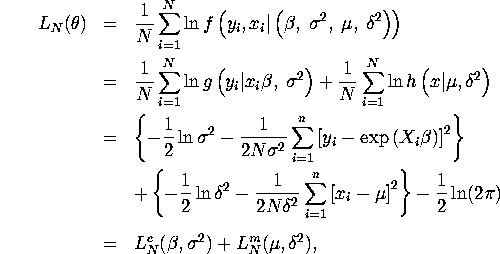
where ![]() denotes the conditional likelihood of the
denotes the conditional likelihood of the ![]() 's
given the
's
given the ![]() 's,
's, ![]() denotes the marginal likelihood
of the
denotes the marginal likelihood
of the ![]() 's,
's,
![]() and
and ![]() .
The separability of parameters in the third and forth equation allows us
to break the estimation problem into two subproblems, which
ordinarily makes the programming considerably
easier and computations considerably faster:
.
The separability of parameters in the third and forth equation allows us
to break the estimation problem into two subproblems, which
ordinarily makes the programming considerably
easier and computations considerably faster:

with FOC's

Note that there is further separability in this first
subproblem: the FOC for ![]() is the same as the FOC for
nonlinear least squares (NLS) estimation of
is the same as the FOC for
nonlinear least squares (NLS) estimation of ![]() in equation (2) above,
ignoring
in equation (2) above,
ignoring ![]() since it doesn't affect the solution for
since it doesn't affect the solution for
![]() . Once we have computed the NLS estimate of
. Once we have computed the NLS estimate of
![]() , we use the second equation to compute
, we use the second equation to compute ![]() as
the sample variance of the estimated NLS residuals.
as
the sample variance of the estimated NLS residuals.
![]()
with FOC's:

respectively. Using attached
Gauss code nlreg.gpr for computing NLS estimates (the sum of
squared errors, derivatives and hessian are coded in the eval.g
procedure) we are able to numerically solve for a
vector ![]() that sets the FOC for
that sets the FOC for ![]() given in
equation (2) above
to zero. There are closed-form expressions for
the MLEs for the remaining parameters:
given in
equation (2) above
to zero. There are closed-form expressions for
the MLEs for the remaining parameters:


Figures 1 and 2 below plot the true and estimated regression
functions for this problem. Figure 1 plots the data points also: we
see that both the true and estimated regression functions are generally
quite close to each other and both go through the middle of the
``data cloud''. However we see that the MLE gives a substantially
downward biased estimate of ![]() and this causes the estimated
regression function to make big divergences from the true regression
function at extreme high and low values of x, say |x| > 4.
However since there
are very few high or low values of x in the sample, the NLS and MLE
are not able to ``penalize'' this divergence: the MLE sets
and this causes the estimated
regression function to make big divergences from the true regression
function at extreme high and low values of x, say |x| > 4.
However since there
are very few high or low values of x in the sample, the NLS and MLE
are not able to ``penalize'' this divergence: the MLE sets
![]() since it helps fit the data around x=0 where
most of the data points are. Figure 2 provides a blow up of Figure
1 without the data points to show you how the estimated regression
function diverges from the truth near x=0. Overall, despite the
misspecification of the heteroscedasticity, the MLE and NLS estimators
seem to do a pretty good job of uncovering the true regression function,
at least for those x's where we have sufficient data. Note that the
data plot indicates heteroscedasticity, since the variance of the data
around the regression function is bigger in the middle of the graph
(near x=0) than at large positive or negative values of x.
since it helps fit the data around x=0 where
most of the data points are. Figure 2 provides a blow up of Figure
1 without the data points to show you how the estimated regression
function diverges from the truth near x=0. Overall, despite the
misspecification of the heteroscedasticity, the MLE and NLS estimators
seem to do a pretty good job of uncovering the true regression function,
at least for those x's where we have sufficient data. Note that the
data plot indicates heteroscedasticity, since the variance of the data
around the regression function is bigger in the middle of the graph
(near x=0) than at large positive or negative values of x.
Since the true model used to generate data1.asc
has heteroscedastic and not homoscedastic error terms ![]() as assumed here, it is easy to
show that the MLE
as assumed here, it is easy to
show that the MLE ![]() of the misspecified model
converges to the
expectation of
of the misspecified model
converges to the
expectation of ![]() .
We can calculate
.
We can calculate ![]() as follows:
as follows:

We leave it to you to show that even though the model is
misspecified, the MLE ![]() converges to
converges to
![]() as
as ![]() . Indeed in this
case we find that
. Indeed in this
case we find that
![]() , which happens to be
almost exactly equal to the ``true'' value.
, which happens to be
almost exactly equal to the ``true'' value.
Recall that the asymptotic distribution of the standardized MLE estimator is given by:
![]()
where ![]() is the Hessian and
is the Hessian and ![]() is the information matrix (both evaluated at
is the information matrix (both evaluated at ![]() ). However the likelihood
is misspecified in this case (due to heteroscedasticity), and
it is easy to verify that the equality of
). However the likelihood
is misspecified in this case (due to heteroscedasticity), and
it is easy to verify that the equality of ![]() does not hold,
so the correct asymptotic
covariance matrix is given by the White ``misspecification consistent''
formula in equation (4) rather than by the inverse of
the information matrix
does not hold,
so the correct asymptotic
covariance matrix is given by the White ``misspecification consistent''
formula in equation (4) rather than by the inverse of
the information matrix ![]() For example, consider the
For example, consider the ![]() block of
block of
![]() , or
, or ![]() :
:
![]()
We see that a sufficient condition for the two expressions above to
equal each other is ![]() for all x, i.e. for the
model to be homoscedastic as you were asked to assume. The failure
of this equality can be a basis for a specification test statistic
that can detect model misspecification which we will discuss in more
detail below.
Note that even despite the misspecification, the separability property implies
that the Hessian is a block diagonal matrix:
for all x, i.e. for the
model to be homoscedastic as you were asked to assume. The failure
of this equality can be a basis for a specification test statistic
that can detect model misspecification which we will discuss in more
detail below.
Note that even despite the misspecification, the separability property implies
that the Hessian is a block diagonal matrix:

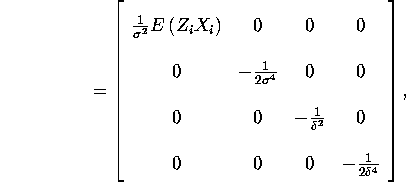
where ![]() .
It is also easy to verify that despite the misspecification
of the heteroscedasicity, the information matrix
.
It is also easy to verify that despite the misspecification
of the heteroscedasicity, the information matrix
![]() is still block diagonal. Block
diagonality of
is still block diagonal. Block
diagonality of ![]() and
and ![]() implies that the covariance matrix of
implies that the covariance matrix of
![]() is block diagonal. One can
see further block diagonality between
is block diagonal. One can
see further block diagonality between ![]() and
and ![]() and
between
and
between ![]() and
and ![]() . This block diagonality is not
just a consequence
of the separability in both the marginal and conditional likelihood
in the parameters describing the mean or conditional mean (
. This block diagonality is not
just a consequence
of the separability in both the marginal and conditional likelihood
in the parameters describing the mean or conditional mean ( ![]() and
and ![]() , respectively) and the variance parameters (
, respectively) and the variance parameters ( ![]() and
and
![]() , respectively). You should verify through direct calculation
that this block diagonality
is a result of the symmetry of the normal distribution, which
implies that
, respectively). You should verify through direct calculation
that this block diagonality
is a result of the symmetry of the normal distribution, which
implies that ![]() , where the conditional
distribution of
, where the conditional
distribution of ![]() given X is
given X is ![]() ,
and similarly, the distribution of
,
and similarly, the distribution of ![]() ,
which implies that
,
which implies that ![]() for any positive odd integer k.
If the normal distribution were not symmetric the block diagonality
property wouldn't hold.
for any positive odd integer k.
If the normal distribution were not symmetric the block diagonality
property wouldn't hold.
Using the block diagonality property, it is easy to compute
the standard errors of the full parameter vector, ![]() .
The covariance matrix of
.
The covariance matrix of ![]() is given by 1/N times
the upper
is given by 1/N times
the upper ![]() block of
block of
![]() and it is easy
to verify that this is the same as the covariance matrix for the
nonlinear least squares estimator for
and it is easy
to verify that this is the same as the covariance matrix for the
nonlinear least squares estimator for ![]() (which is also
numerically identical to the MLE) that is output from
the nlreg.gpr program. By working with equation (4), you
can show that the
estimated variance of
(which is also
numerically identical to the MLE) that is output from
the nlreg.gpr program. By working with equation (4), you
can show that the
estimated variance of ![]() is given by
is given by ![]() where
where ![]() is the sample
analog of the fourth central moment of
is the sample
analog of the fourth central moment of ![]() :
:
![]()
There is a similar formula for the estimated variance of
![]() . We have
. We have ![]() , so
the estimated standard error of
, so
the estimated standard error of ![]() is 0.036. The estimated
standard error of
is 0.036. The estimated
standard error of ![]() is
is ![]() .
.
![]()
We compare White's misspecification consistent estimate to the inverse of information:

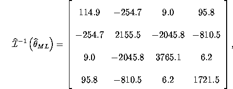
where all the estimates are given from the results of eval.g.
Following White (``Maximum Likelihood Estimation
of Misspecified Models'' Econometrica 1982)
we can construct a formal hypothesis test statistic using the
difference between the estimates of the
upper diagonal elements of ![]() and the corresponding
elements of
and the corresponding
elements of ![]() . This statistic should be small
if the null hypothesis of correct specification is true (since
. This statistic should be small
if the null hypothesis of correct specification is true (since
![]() in that case), and large if the
model is misspecified (since it is not necessarily
true that
in that case), and large if the
model is misspecified (since it is not necessarily
true that ![]() is the model is
misspecified). The large difference
in the two difference estimates of the covariance matrix for
is the model is
misspecified). The large difference
in the two difference estimates of the covariance matrix for
![]() suggests that
suggests that ![]() and
and ![]() are different, and hence that the model is misspecified. However
we did not actually compute the actual test statistic to see at
what level of significance
null would actually be rejected (i.e. to compute the
marginal signficance level of the test statistic)
since we didn't expect you to know about
this particular specification test statistic at this stage of the
course.
are different, and hence that the model is misspecified. However
we did not actually compute the actual test statistic to see at
what level of significance
null would actually be rejected (i.e. to compute the
marginal signficance level of the test statistic)
since we didn't expect you to know about
this particular specification test statistic at this stage of the
course.
![]()
where ![]() , then it is easy to see
that the
, then it is easy to see
that the ![]() are conditionally lognormally distributed
so it is valid to take log transformation and estimate
are conditionally lognormally distributed
so it is valid to take log transformation and estimate ![]() by OLS:
by OLS:
![]()
.
It would not difficult to show that the OLS estimates of the
log-linearized model are actually the maximum likelihood estimates
of the original lognormal specification (make sure you understand
this by writing down the lognormal likelihood function and verifying
what we just said is true)! However the error
term for the specification of Model I in part (a) is additive and
not multiplicative, and so the log transformation is generally not
valid. Indeed, there is a positive probability of observing negative
realizations of ![]() , something that has zero probability under the
lognormal specification. Thus, to even do OLS one must screen out
all
, something that has zero probability under the
lognormal specification. Thus, to even do OLS one must screen out
all ![]() pairs where
pairs where ![]() is negative, something that is
generally not a good idea. When one does OLS on this nonrandomly
selected subsample, it is not surprising that the estimates are
highly biased:
is negative, something that is
generally not a good idea. When one does OLS on this nonrandomly
selected subsample, it is not surprising that the estimates are
highly biased:
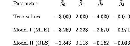
We can show analytically why the OLS estimates for Model II will be inconsistent when the true model is Model I with additive normal errors rather than multiplicative lognormal errors. After screening out negative y's, the OLS estimator solves:
![]()
As ![]() , we can show that the right hand side of the above
equation converges uniformly to
, we can show that the right hand side of the above
equation converges uniformly to
![]()
In general the ![]() that minimizes the expression above is not
the same as the
that minimizes the expression above is not
the same as the ![]() that minimizes
that minimizes
![]()
which is the true ![]() when the conditional mean function
when the conditional mean function
![]() is correctly specified.
Therefore, we conclude that the probability limits for
is correctly specified.
Therefore, we conclude that the probability limits for ![]() 's
from the two different models( Model I and Model II) are not the same.\
's
from the two different models( Model I and Model II) are not the same.\
![]()
where as before ![]() and
and ![]() is a
conformable
is a
conformable ![]() parameter vector. We see substantial
evidence of heteroscedasticity, confirming our earlier visual
impression in looking at the data in figure 1. The estimated
conditional variance function looks concave and symmetric w.r.t.
y-axis, almost like a normal density. Table 3
summarizes the estimation results. According to table 3, the regression
coefficient for the quadratic term is significant and seems to
dominate the form of the heteroscedasticity plotted in figure 3.
Figure 4 does a blow up, plotting the estimated and true conditional
variance functions.
parameter vector. We see substantial
evidence of heteroscedasticity, confirming our earlier visual
impression in looking at the data in figure 1. The estimated
conditional variance function looks concave and symmetric w.r.t.
y-axis, almost like a normal density. Table 3
summarizes the estimation results. According to table 3, the regression
coefficient for the quadratic term is significant and seems to
dominate the form of the heteroscedasticity plotted in figure 3.
Figure 4 does a blow up, plotting the estimated and true conditional
variance functions.

Some students may have used simple OLS, estimating a specification like
![]()
rather than the
exponential specification in equation (7).
This is also OK since we weren't specific about what type
of tool to use to check for heteroscedasticity. The only
disadvantage of the OLS specification in (8) over the exponential
specification in (7) is that the latter doesn't guarantee that
![]() for all x. However
we find that even in the linear specification most
of the predicted
for all x. However
we find that even in the linear specification most
of the predicted ![]() values are indeed positive.
Figure 4 compares the predicted values of
values are indeed positive.
Figure 4 compares the predicted values of ![]() using both
specifications, and we can see that the negative predicted values
of
using both
specifications, and we can see that the negative predicted values
of ![]() occur at the extreme high and low values of
the observed x's.
occur at the extreme high and low values of
the observed x's.
![]()
where ![]() , and
, and
![]() .
We want to consider simultaneous or ``full information
maximum likelihood'' (FIML) estimation of the parameter vector
.
We want to consider simultaneous or ``full information
maximum likelihood'' (FIML) estimation of the parameter vector
![]() . The log-likelihood function
. The log-likelihood function
![]() is given by:
is given by:
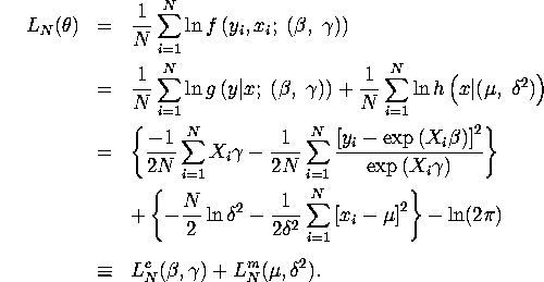
where ![]() and
and ![]() The gradients of
The gradients of ![]() with respect to
with respect to
![]() are:
are:

The gradients for ![]() with
respect to
with
respect to ![]() are the same as
in part (a).
The hessian matrix for
are the same as
in part (a).
The hessian matrix for ![]() with respect to
with respect to ![]() is given by:
is given by:

It is easy to verify (using the law of iterated expectations)
that when ![]() ,
the expectation of
,
the expectation of
![]() ,
i.e. we have block diagonality between the
,
i.e. we have block diagonality between the ![]() and
and ![]() parameters (assuming the model is correctly specified). Similarly
one can verify that the
parameters (assuming the model is correctly specified). Similarly
one can verify that the ![]() block of the information
matrix
block of the information
matrix ![]() is zero. This implies that the asymptotic
covariance between the maximum likelihood
estimates
is zero. This implies that the asymptotic
covariance between the maximum likelihood
estimates ![]() and
and ![]() is zero, so they
are asymptotically independently distributed. This independence suggests
the following 2-step procedure to obtain initial consistent estimates
of
is zero, so they
are asymptotically independently distributed. This independence suggests
the following 2-step procedure to obtain initial consistent estimates
of ![]() : 1) estimate
: 1) estimate ![]() by NLS (see
attached Gauss code eval_nls.g and shell program
nlreg.gpr), 2) use the
estimated squared residuals
by NLS (see
attached Gauss code eval_nls.g and shell program
nlreg.gpr), 2) use the
estimated squared residuals ![]() to estimate the
to estimate the
![]() parameters by NLS using the exponential specification in
equation (7). We did this using the same eval_nls.g
procedure we used for step 1, with a slight modification of
nlreg.gpr to substitute
parameters by NLS using the exponential specification in
equation (7). We did this using the same eval_nls.g
procedure we used for step 1, with a slight modification of
nlreg.gpr to substitute ![]() instead
of
instead
of ![]() as the dependent variable in the regression.
as the dependent variable in the regression.
However we can do even better than this. We can do a 3rd step,
weighted NLS or feasible generalized least squares (FGLS) estimation of
![]() using the estimated conditional variance
using the estimated conditional variance
![]() from step 2 as weights.
The procedure eval_fgls.g provides the code to do the FGLS
estimation.
Due to the block diagonality property, it is not hard to show
that the FGLS estimates of
from step 2 as weights.
The procedure eval_fgls.g provides the code to do the FGLS
estimation.
Due to the block diagonality property, it is not hard to show
that the FGLS estimates of ![]() have the same asymptotic
distribution as the MLE: i.e. FGLS is asymptotically efficient
in this case. To see this, note that the gradient and hessian of
have the same asymptotic
distribution as the MLE: i.e. FGLS is asymptotically efficient
in this case. To see this, note that the gradient and hessian of
![]() with respect to
with respect to ![]() is the same as the
gradient and hessian for the following FGLS criterion function:
is the same as the
gradient and hessian for the following FGLS criterion function:

We know that the block diagonality property implies that as
long as ![]() is any consistent estimator of
is any consistent estimator of ![]() that
a solution
that
a solution ![]() to the FOC
to the FOC ![]() is asymptotically efficient. But since this is also the FOC
for the FGLS estimator (10), it follows that
is asymptotically efficient. But since this is also the FOC
for the FGLS estimator (10), it follows that ![]() is also an asymptotically efficient estimator, i.e. it attains not
only the Chamberlain efficiency bound for condition moment restrictions,
but the Cramer-Rao lower bound as well. It is not hard to show that
these two bounds coincide in this case: make sure
you understand this by verifying the equality yourself.
is also an asymptotically efficient estimator, i.e. it attains not
only the Chamberlain efficiency bound for condition moment restrictions,
but the Cramer-Rao lower bound as well. It is not hard to show that
these two bounds coincide in this case: make sure
you understand this by verifying the equality yourself.
It is not apparent that the ![]() obtained from the 4th step
of our estimation procedure which regresses the squared residuals
from the FGLS estimation in step 3 on
obtained from the 4th step
of our estimation procedure which regresses the squared residuals
from the FGLS estimation in step 3 on ![]() will be
asymptotically efficient since the first order condition for
will be
asymptotically efficient since the first order condition for ![]() from maximizing
from maximizing ![]() with respect to
with respect to ![]() does not appear to be the same as the FOC for
does not appear to be the same as the FOC for ![]() from the
nonlinear regression in step 4 of our suggested estimation procedure.
So to get fully efficient estimates, we can use
from the
nonlinear regression in step 4 of our suggested estimation procedure.
So to get fully efficient estimates, we can use ![]() as starting values for direct
FIML estimation of the full parameter vector
as starting values for direct
FIML estimation of the full parameter vector ![]() using
using
![]() . The procedure eval_fiml.g and the
shell program mle.gpr implement full maximum likelihood estimation
of Model III (note we have also provided the
procedure hesschk.g to allow you to compare numerical
and analytically calculated values of the hessian matrix, verifying
that the analytic formulas for the hessian matrix given above are
correct). This full model is rather delicate and we were unable to
get it to converge starting from
. The procedure eval_fiml.g and the
shell program mle.gpr implement full maximum likelihood estimation
of Model III (note we have also provided the
procedure hesschk.g to allow you to compare numerical
and analytically calculated values of the hessian matrix, verifying
that the analytic formulas for the hessian matrix given above are
correct). This full model is rather delicate and we were unable to
get it to converge starting from ![]() . However we
had no problems with convergence starting from
. However we
had no problems with convergence starting from
![]() . Table 4 below
compares the FGLS and MLE estimates.
. Table 4 below
compares the FGLS and MLE estimates.
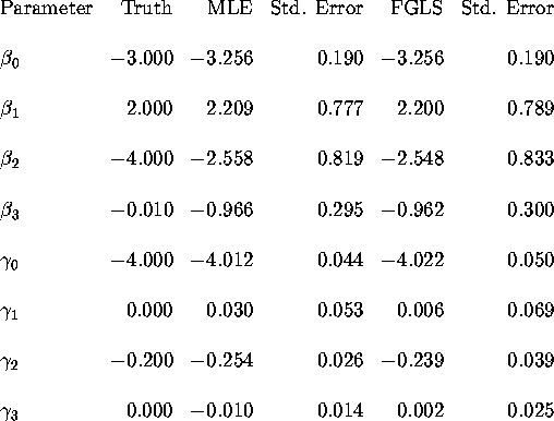
We see that the FIML and FGLS estimates of ![]() are very close
to each other and the standard errors are nearly identical, as we
would expect from the theoretical result shown above that the
FGLS estimator of
are very close
to each other and the standard errors are nearly identical, as we
would expect from the theoretical result shown above that the
FGLS estimator of ![]() is asymptotically efficient. There
are more significant differences in the FIML and FGLS estimates
of
is asymptotically efficient. There
are more significant differences in the FIML and FGLS estimates
of ![]() . In particular the standard errors of the FGLS estimates
are significantly larger than the FIML estimates of
. In particular the standard errors of the FGLS estimates
are significantly larger than the FIML estimates of ![]() , which
suggests that the FGLS estimates are not asymptotically efficient.
Students should be able to verify that this is the case by
deriving analytic formulas for the asymptotic covariance matrix
for the MLE and FGLS estimators of
, which
suggests that the FGLS estimates are not asymptotically efficient.
Students should be able to verify that this is the case by
deriving analytic formulas for the asymptotic covariance matrix
for the MLE and FGLS estimators of ![]() .
.