


Next: About this document ...
Econ 551: Lecture Note 9
Asymptotic Properties of Nonlinear Estimators
Professor John Rust
Background: So far in Econ 551 we have focused
on the asymptotic properties of nonlinear least squares and maximum
likelihood estimators under the IID sampling assumption
(i.e. that the data
 are
independent and identically distributed draws from some unknown
joint population distribution F(y,x)). However this basic
asymptotic framework can be generalized to a much wider class
of M-estimators (where ``M'' is intended as a mnemonic
for ``Maximization'') where the estimator
are
independent and identically distributed draws from some unknown
joint population distribution F(y,x)). However this basic
asymptotic framework can be generalized to a much wider class
of M-estimators (where ``M'' is intended as a mnemonic
for ``Maximization'') where the estimator
 of some unknown parameter vector
  is the solution
to an optimization problem, just as in least squares or
maximum likelihood. We can also dispense with the IID
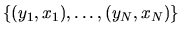
sampling assumption and allow the data
to be a realization of a strictly stationary and ergodic stochastic
process. These notes will also discuss the closely related class of
Z estimators and GMM estimators.
is the solution
to an optimization problem, just as in least squares or
maximum likelihood. We can also dispense with the IID
sampling assumption and allow the data
to be a realization of a strictly stationary and ergodic stochastic
process. These notes will also discuss the closely related class of
Z estimators and GMM estimators.
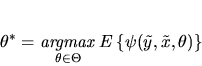
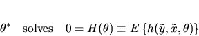
M-Estimators These are defined in terms of
a population optimization condition for the ``true parameter'' ,
i.e. we assume there is some function
 whose expectation
is uniquely maximized at the ``true'' value of the parameter, :
whose expectation
is uniquely maximized at the ``true'' value of the parameter, :
 |
(1) |
where the expectation is taken with respect to the invariant
distribution of (yt,xt) (which doesn't depend on t due to the
assumption of strict stationarity), and the function  is
twice continuously differentiable in
is
twice continuously differentiable in  for each
(y,x) and measurable in (y,x) for each .
We assume the
parameter space
for each
(y,x) and measurable in (y,x) for each .
We assume the
parameter space  is a compact subset of RK and that
is uniquely identified as an interior point of .
is a compact subset of RK and that
is uniquely identified as an interior point of .
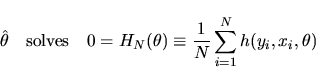
The M-estimator is then given
by a sample analog optimization condition for
.
That is,
for any strictly stationary and ergodic stochastic process,
averages of functions of
the values of the process converge to the ``long run expectation'',
i.e. the expectation with respect to the marginal or invariant
distribution of the process, we can apply the Analogy principle
and compute
as
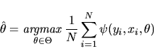 |
(2) |
Note that whether we are taking min or max is inessential, since
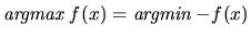 .
Note that
the class of M-estimators encompass both
maximum likelihood (
.
Note that
the class of M-estimators encompass both
maximum likelihood (
![$\psi(y,x,\theta)=\log[f(y\vert x,\theta)]$](img11.gif) )
and linear and nonlinear
least squares (
)
and linear and nonlinear
least squares (
![$\psi(y,x,\theta)=-[y-f(x,\theta)]^2$](img12.gif) )
as special cases.
)
as special cases.
Z-Estimators There is a closely related class of estimators
calls Z-Estimators (with the ``Z'' denoting ``Zero'') where
the parameters are solutions or zeros to system of nonlinear equations.
Generally the first order condition to an M-estimator defines an
associated Z-estimator. Given a function
 ,
we
assume the true parameter
is the unique solution to the following
population unconditional moment restrictions or orthogonality condition
,
we
assume the true parameter
is the unique solution to the following
population unconditional moment restrictions or orthogonality condition
 |
(3) |
The Z-estimator
is defined as a solution to the sample
analog of the population moment condition in equation (3):
 |
(4) |
Here h is a
 vector functions of
 .
Note that an M-estimator with function
implies
an associated Z-estimator with function
.
Note that an M-estimator with function
implies
an associated Z-estimator with function
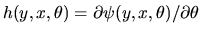 .
.
GMM Estimators and Minimum Distance Estimators
Given a Z-estimator one can
define an associated estimator, a GMM estimator (for
Generalized Methods of Moments) that is basically similar to an
M-estimator, or more precisely, a type of Minimum Distance
Estimator.
If there are more orthogonality conditions than parameters, i.e.
if J > K, then it will generally not be possible to find an exact
zero to the sample orthogonality condition (4) and so it is convenient
to transform the Z-estimator into an M-estimator using a
 positive definite weighting matrix W. In the limiting
population case, it is easy to see that
is a solution
to (3) if and only if
is the unique minimizer of
positive definite weighting matrix W. In the limiting
population case, it is easy to see that
is a solution
to (3) if and only if
is the unique minimizer of
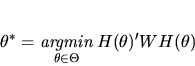 |
(5) |
Once again we appeal to the analogy principle to define the GMM
estimator by replacing  with its sample analog
 and replacing W by any positive definite (possibly
stochastic) weighting matrix WN that converges in probability
to W:
and replacing W by any positive definite (possibly
stochastic) weighting matrix WN that converges in probability
to W:
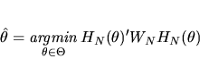 |
(6) |
This estimator is also known as a minimum distance estimator
since the quadratic form x' WN x defines (the square of)
a norm or distance function on RJ, (i.e. the distance
between two vectors x and y in RJ under this norm is
sqrt (x-y)' WN (x-y)). Thus, the GMM estimator is defined as the
parameter estimate
that make the sample orthogonality
conditions
as close as possible to zero in this norm.
-
- Example 1 Consider the linear model
 .
Note that OLS esimator
is a type of GMM estimator with
the orthogonality condition
.
Note that OLS esimator
is a type of GMM estimator with
the orthogonality condition
 when
when
 .
In this case the parameter
is
said to be just-identified since there are
as many orthogonality conditions J as parameters K.
Assuming that the
.
In this case the parameter
is
said to be just-identified since there are
as many orthogonality conditions J as parameters K.
Assuming that the
 matrix
 is
invertible, the population moment condition can be solved
to show that
must equal the standard formula for the
coefficients of the best linear predictor of
is
invertible, the population moment condition can be solved
to show that
must equal the standard formula for the
coefficients of the best linear predictor of  given
given
 :
:
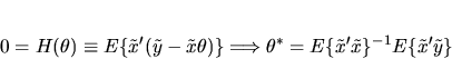 |
(7) |
It is straightforward to show that if the matrix
 is invertible, that the GMM estimator
for this
moment condition reduces to the OLS estimator,
is invertible, that the GMM estimator
for this
moment condition reduces to the OLS estimator,
![$\hat\theta =
[\sum_{i=1}^N x_i' x_i]^{-1} [\sum_{i=1}^N x_i' y_i]$](img33.gif) regardless
of the choice of a positive weighting matrix WN since the
OLS estimates set
regardless
of the choice of a positive weighting matrix WN since the
OLS estimates set
 identically.
-
- Exercise 1 Consider a linear structural model
but where some
of the x variables are suspected of being endogenous,
i.e.
 .
Suppose there
are
.
Suppose there
are  instrumental variables z, i.e. the
(y,x,z) satisfy the following orthogonality condition
at :
instrumental variables z, i.e. the
(y,x,z) satisfy the following orthogonality condition
at :
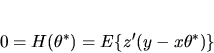 |
(8) |
Show that the GMM estimator for this orthogonality condition
coincides with the two stage least squares estimator.
Next: About this document ...
John Rust
2001-03-19