Spring 1997 John Rust
Economics 551b 37 Hillhouse, Rm. 27
PROBLEM SET 1: SOLUTIONS
Bayesian Basics
QUESTION 1
Ans: ![]() median of
median of ![]() .
.
Proof:
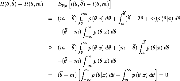
Let ![]() be any number such that
be any number such that ![]() .
.
Then

Since ![]() when
when ![]() , the following result can be obtained:
, the following result can be obtained:

Last equality holds since
![]()
by the definition of median.
Inequality will be an equality if, and only if ,
![]()
This implies that ![]() is also a median.
is also a median.
A similar proof can also be given when ![]() is any number
such that
is any number
such that ![]() .
.
Therefore
![]()
QUESTION 2
Ans: ![]() th
percentile of
th
percentile of ![]() .
.
Proof:
Let ![]() be any number such that
be any number such that ![]() .
.
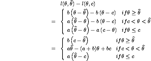
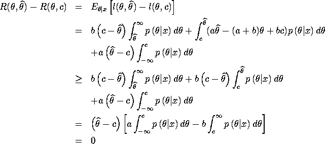
Then

Since ![]() when
when ![]() , the following result can be obtained:
, the following result can be obtained:

Last equality holds since

by the definition of ![]() th percentile.
th percentile.
Inequality will be an equality if, and only if ,
![]()
This implies that ![]() is also a
is also a ![]() th
percentile.
th
percentile.
A similar proof can also be given when ![]() is any number
such that
is any number
such that ![]() .
.
Therefore
![]()
QUESTION 3
From definition of posterior distribution,
![]()

Since ![]() ,
,
Normalizer is
![]()
Therefore,
![]()
which is also a Beta distribution ![]() .
.
QUESTION 4
Sample GAUSS program:
/* BETAPLOT.GPR: program to plot posterior distributions from
** a Bernoulli-Beta conjugate family.
** John Rust, Yale University, January, 1997 */
library pgraph;
graphset;
x=seqa(.001,.001,999); /* points on the x axis to plot prior distribution */
a=1; /* set hyperparameters of Beta distribution */
b=1;
/* now compute beta distribution over the grid of x points */
betaden=gamma(a+b)*(x94(a-1)).*((1-x)94(b-1))/(gamma(a)*gamma(b));
truethet=.3;
/* now compute beta distribution over the grid of x points */
randat=rndu(500,1);
n=10;
d=(randat[1:n].<=truethet);
a1=a+sumc(d);
b1=b+n-sumc(d);
postden1=gamma(a1+b1)*(x94(a1-1)).*((1-x)94(b1-1))/(gamma(a1)*gamma(b1));
n=100;
d=(randat[1:n].<=truethet);
a1=a+sumc(d);
b1=b+n-sumc(d);
postden2=gamma(a1+b1)*(x94(a1-1)).*((1-x)94(b1-1))/(gamma(a1)*gamma(b1));
n=150;
d=(randat[1:n].<=truethet);
a1=a+sumc(d);
b1=b+n-sumc(d);
postden3=gamma(a1+b1)*(x94(a1-1)).*((1-x)94(b1-1))/(gamma(a1)*gamma(b1));
/* Now plot out the prior and posterior densities */
#IFUNIX /* this part is only necessary if you are running on
a Unix system (like I am). It creates the window
where the plot is printed. You don't need to worry
about this code for Dos/Windows systems */
let v = 100 100 640 480 0 0 1 6 15 0 0 2 2;
wxy = WinOpenPQG(v,''XY Plot'',''XY'');
call WinSetActive(wxy);
#ENDIF
_pdate='''';
title(''Beta-Bernoulli Prior and Posterior Densities'');
ylabel(''Density at x'');
xlabel(''X value'');
/* the following commands put legends on the plot so you
can tell which density curve is which */
_plegctl=212651264.21264.7;
_plegstr=''Beta prior density (a=1, b=1)000Beta posterior density (n=10)'';
_plegstr=_plegstr$+''000Beta posterior density (n=100)000Beta posterior density (n=150)'';
/* these commands specify the plotting bounds for the
x and y axes */
y=betaden126postden1126postden2126postden3;
xtics(0,1,.1,3);
ytics(0,maxc(maxc(y)),1,1);
/* finally this command actually does the plot */
xy(x,y);
#IFUNIX
call WinSetActive(1);
#ENDIF