Spring 1997 John Rust
Economics 551b 37 Hillhouse, Rm. 27
MIDTERM EXAM: SOLUTIONS
QUESTION 1
Seemingly unrelated regression estimator is identical to OLS estimator when
regressors of all equations are identical. (Therefore you can check your SUR
program by comparing SUR estimates and OLS estimates. Now, you have your own
SUR program which you can use to estimate models with different
regressors(!).)
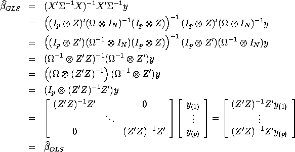
We know that GLS estimator of SUR model is unbiased and efficient and can be written as
![]()
where


If we introduce the regressor matrices stacked by equation by equation instead of observation by observation (see solution of Q4 in Problem set 3), this estimator can be rewritten as:
![]()
where


Suppose we have identical regressors, ![]() .
.

Then

1. ![]() should be constant among
equations.
should be constant among
equations.
2. SUR-GLS estimator or OLS estimator equation by equation from argument above.
3. Construct sample covariance matrix from OLS residuals.
4. See the calculation above.
5. I apologize for asking you to do Gibbs sampling for the full
set of 63 securities: this isn't really feasible on most computers
in a reasonable amount of time. With 63 securities it takes
special programming to be able to run the Gibbs sampling program
without using a great deal of memory space. Even when you do this the
program still takes quite a bit of cpu time for the
ordinary Pentium cpus in the Statlab. However if you choose a
few securities from the data set, say 3 or 4 stocks, then Gibbs
sampling runs reasonably quickly. Any student who just did this
part using just a subset of securities in stockdat
received full credit. All students who
even attempted to do this part received generous
partial credit, and nearly full credit if
you developed a computer program to carry out the
Gibbs sampling that looked correct and included it
in your anwer, regardless of whether it
actually worked for the problem using all 63 securities.
I was more interested in getting students
to write code for this problem rather than seeing actual output
since the output will differ from person to person by the nature
of the Gibbs sampling algorithm. I have written a program
surgibbs.gpr that carries out Gibbs sampling for
seemingly unrelated regression models and have the code set up
to do Gibbs sampling with 3 stocks from stockdat so you
can see how it runs. The program comes with 2 procedures,
set_hp.g and get_dat.g which you can modify to
use the software for other problems, including an artificial
problem where you know the true ![]() and
and ![]() parameters
in advance (this is useful as a check that the program is
coded correctly).
parameters
in advance (this is useful as a check that the program is
coded correctly).
QUESTION 2
Let ![]() be the number of times which outcome k occured in all sample.
be the number of times which outcome k occured in all sample.
![]()
With
![]()
the joint distribution of ![]() can be
written as
can be
written as
![]()
1. Since log likelihood function is

MLE ![]() (for
(for ![]() ) can be derived from
) can be derived from
![]()
The solution to this system is
![]()
2.Since
![]()
![]()
Therefore ![]() is an unbiased estimator.
is an unbiased estimator.
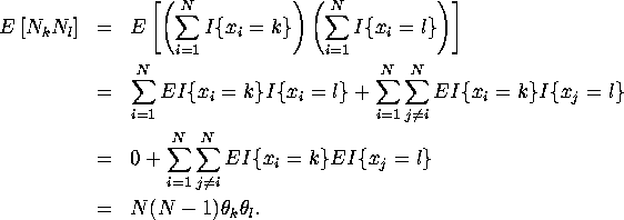
3.

![]()

For ![]()

Note ![]() since at least one of
since at least one of ![]() and
and ![]() must be zero.
must be zero.
![]()

Therefore

4.
For k=l
![]()

For ![]()
![]()


5. MLE can be proved to be efficient if it has a variance equal to
Cramer-Rao lower bound. You can easily show ![]() by verifying
by verifying ![]() .
.
6. Run the program dirichlet.gpr (which in turn calls
a procedure setparm.g) available
on the Econ 551 Web page. This program does the calculations required
in part 6, i.e. it compares that posterior probability that ![]() (a draw from the Dirichlet posterior) is within a ball of radius
.01 of the true parameter
(a draw from the Dirichlet posterior) is within a ball of radius
.01 of the true parameter ![]() . I calculate this probability
by simulation. Since this posterior probability is simulated, and since
the data used to form the posterior is simulated, it makes no sense
to report numbers here since they vary from run to run. The important
part of this exercise is to verify that the simulated probability from
the exact posterior is very close to the probability
calculated from the normal approximation to
the posterior.
. I calculate this probability
by simulation. Since this posterior probability is simulated, and since
the data used to form the posterior is simulated, it makes no sense
to report numbers here since they vary from run to run. The important
part of this exercise is to verify that the simulated probability from
the exact posterior is very close to the probability
calculated from the normal approximation to
the posterior.
7. First, notice that the full ![]() vector
vector
![]() is not identified: you can add a
constant
is not identified: you can add a
constant ![]() to each component of
to each component of ![]() and the probability
in (5) will be unchanged. Therefore I impose an arbitrary normalization
that
and the probability
in (5) will be unchanged. Therefore I impose an arbitrary normalization
that ![]() and our problem reduces to the estimation of the
unrestricted
and our problem reduces to the estimation of the
unrestricted ![]() vector
vector ![]() .
Another arbitrary but convenient normalization is:
.
Another arbitrary but convenient normalization is:
![]()
Under the first normalization, one can show that there is a
one to one mapping between the K-1 ![]() parameters and the
K-1
parameters and the
K-1 ![]() parameters. Thus, the by the invariance of
maximum likelihood, it is easy to see that
parameters. Thus, the by the invariance of
maximum likelihood, it is easy to see that
![]() will be given by the unique solution to
the K-1 system of equations
will be given by the unique solution to
the K-1 system of equations

Under the second normalization we can get an explicit representation:
![]() .
Since
.
Since ![]() is an unbiased estimator as was verified in part 2 above, it follows
from Jensen's inequality that
is an unbiased estimator as was verified in part 2 above, it follows
from Jensen's inequality that ![]() will be a downward
biased estimator of
will be a downward
biased estimator of ![]() . Due to the
presence of bias and the arbitrariness of the identifying
normalization, it is difficult to determine whether the
MLE
. Due to the
presence of bias and the arbitrariness of the identifying
normalization, it is difficult to determine whether the
MLE ![]() attains the generalized Cramer-Rao lower bound
in finite samples. However we know that this is a regular
problem, so the MLE is asymptotically unbiased and efficient, and
so does attain the Cramer-Rao lower bound asymptotically. Under
the first identifying normalization,
attains the generalized Cramer-Rao lower bound
in finite samples. However we know that this is a regular
problem, so the MLE is asymptotically unbiased and efficient, and
so does attain the Cramer-Rao lower bound asymptotically. Under
the first identifying normalization, ![]() , it is
easy to calculate the information matrix in this case and
verify that it is the same as the inverse of the information
matrix for
, it is
easy to calculate the information matrix in this case and
verify that it is the same as the inverse of the information
matrix for ![]() . This should not be surprising, since the
. This should not be surprising, since the ![]() parameters are an inverse transformation of the
parameters are an inverse transformation of the ![]() parameters
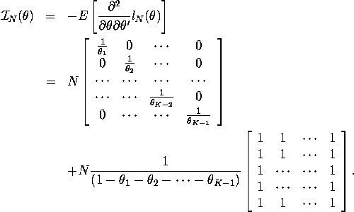
in this case. I present the derivation below. The information matrix
parameters
in this case. I present the derivation below. The information matrix
![]() is given by:
is given by:
![]()
But we have

and
![]()
where ![]() is a
is a ![]() vector of zeros with a 1 in the
vector of zeros with a 1 in the
![]() place. Substituting this into the equation for
place. Substituting this into the equation for
![]() above we get
above we get
![]()
You can verify that this matrix is the same as the covariance matrix
for ![]() given above, and as already
demonstrated, this covariance matrix is the inverse of the information
matrix for
given above, and as already
demonstrated, this covariance matrix is the inverse of the information
matrix for ![]() . So the information matrix for
. So the information matrix for ![]() is the
inverse of the information matrix for
is the
inverse of the information matrix for ![]() .
.
QUESTION 3

For the first term in the last inequality, ![]() with probability 1 by assumption. For the
second term, H continuous and
with probability 1 by assumption. For the
second term, H continuous and ![]() with
probability 1, together implies
with
probability 1, together implies ![]() with
probability 1 by continuous mapping theorem.
with
probability 1 by continuous mapping theorem.
Therefore ![]() with probability 1.
with probability 1.
QUESTION 4. The Econ 551 web has Gauss programs for computing maximum likelihood estimates of the multinomial logit model plus the shell programs for running maximum likelihood. I have also posted evalbprob.g which is the procedure for computing the likelihood and derivatives for the biniomial probit model. You can run each of these programs to get the maximum likelihood estimates for the models. I have posted the estimation results for each of these programs on the Econ 551 web page.
![]()
That is, ![]() is an indicator for the event
that the decision
is an indicator for the event
that the decision ![]() taken by person i is alternative
j should equal the choice probability
taken by person i is alternative
j should equal the choice probability ![]() plus
an error term,
plus
an error term, ![]() . Since
. Since ![]() is the
conditional expectation of
is the
conditional expectation of ![]() , the error term
must have mean zero. Therefore we can ``test'' the model both in sample
and out of sample by computing the mean prediction errors, and
seeing how close they are to zero:
, the error term
must have mean zero. Therefore we can ``test'' the model both in sample
and out of sample by computing the mean prediction errors, and
seeing how close they are to zero:
![]()
Under standard regularity conditions,
if the null hypothesis that the model is correctly specified,
![]() where
where ![]() is the unconditional variance of
is the unconditional variance of
![]() . This can be used to form a test statistic. However
we need to replace the unknown true
. This can be used to form a test statistic. However
we need to replace the unknown true ![]() with the
maximum likelihood estimate
with the
maximum likelihood estimate ![]() and then determine
the asymptotic distribution of the corresponding
and then determine
the asymptotic distribution of the corresponding ![]() statistic,
doing an ``Amemiya correction'' for the fact that we are
using an estimated value
statistic,
doing an ``Amemiya correction'' for the fact that we are
using an estimated value ![]() to construct
to construct ![]() and
we need to account for this extra estimation error in the derivation
of the asymptotic distribution of the test statistic. Once we do
this, we can use the
and
we need to account for this extra estimation error in the derivation
of the asymptotic distribution of the test statistic. Once we do
this, we can use the ![]() statistic
as a ``moment condition'' and set up a hypothesis
test to see how well this moment condition is satisfied. Indeed,
since
statistic
as a ``moment condition'' and set up a hypothesis
test to see how well this moment condition is satisfied. Indeed,
since ![]() , we can
construct an entire family of moment conditions that should be
zero if the model is correctly specified. We can actually
construct an entire vector of such test statistics, one for
each alternative
, we can
construct an entire family of moment conditions that should be
zero if the model is correctly specified. We can actually
construct an entire vector of such test statistics, one for
each alternative ![]() and for each instrument
X that we use in forming the moment conditions. Later in
Econ 551 we will show how to test all these moment conditions
simultaneously using a single Chi-square goodness of fit
statistic. This statistic would be the analog of the
and for each instrument
X that we use in forming the moment conditions. Later in
Econ 551 we will show how to test all these moment conditions
simultaneously using a single Chi-square goodness of fit
statistic. This statistic would be the analog of the
![]() . It is important to
note that we should expect the model to fit better within sample
than out-of-sample since maximum likelihood is designed to
choose parameters to fit a given sample of data as well as possible.
In fact, with a full set of alternative specific dummies, it
is easy to show that the mean prediction error for each
alternative is identically zero within sample, i.e.
. It is important to
note that we should expect the model to fit better within sample
than out-of-sample since maximum likelihood is designed to
choose parameters to fit a given sample of data as well as possible.
In fact, with a full set of alternative specific dummies, it
is easy to show that the mean prediction error for each
alternative is identically zero within sample, i.e. ![]() .
However
.
However ![]() is not necessarily zero if we use out of
sample data, i.e. if we estimate
is not necessarily zero if we use out of
sample data, i.e. if we estimate ![]() using
using
![]() for
for ![]() and then construct
and then construct ![]() using
using ![]() for
for ![]() . The program
tnlest.gpr presents the mean prediction errors (by alternative)
both in-sample and out-of-sample (where in sample
. The program
tnlest.gpr presents the mean prediction errors (by alternative)
both in-sample and out-of-sample (where in sample ![]() was
constructed from the first N=1500 observations and the out-of-sample
was
constructed from the first N=1500 observations and the out-of-sample
![]() was constructed from
was constructed from ![]() and the
remaining M=500 observations in the data set. The results verify
that the mean prediction errors are zero (modulo rounding error)
within sample, but are non-zero out of sample. Later in the
course we will post software for doing
and the
remaining M=500 observations in the data set. The results verify
that the mean prediction errors are zero (modulo rounding error)
within sample, but are non-zero out of sample. Later in the
course we will post software for doing ![]() specification
tests using the residuals from the estimated choice model.
specification
tests using the residuals from the estimated choice model.
![]()

QUESTION 5. The fact that ![]() implies that
implies that ![]() . But from earlier in the
semester we know that the median is the solution to the minimization
problem
. But from earlier in the
semester we know that the median is the solution to the minimization
problem
![]()
Conditioning on X it follows that ![]() is the solution to
the problem
is the solution to
the problem
![]()
so unconditionally we have:
![]()
Under assumptions of no multicollinearity between the columns
of ![]() ,
, ![]() will be the unique solution to the
above minimization problem and hence is uniquely identified.
Assume the observations
will be the unique solution to the
above minimization problem and hence is uniquely identified.
Assume the observations ![]() are IID. By the
uniform strong law of large numbers we have with probability 1:
are IID. By the
uniform strong law of large numbers we have with probability 1:
![]()
where ![]() is a compact set in
is a compact set in ![]() containing
containing ![]() .
Since
.
Since ![]() is uniquely minimized
at
is uniquely minimized
at ![]() , it follows that
, it follows that ![]() with
probability 1. For further details on the asymptotic properties of
the LAD estimator (including a derivation of the
asymptotic distribution of the LAD estimator),
see Koenker and Bassett, ``Regression Quantiles''
in the January 1978 Econometrica.
with
probability 1. For further details on the asymptotic properties of
the LAD estimator (including a derivation of the
asymptotic distribution of the LAD estimator),
see Koenker and Bassett, ``Regression Quantiles''
in the January 1978 Econometrica.