Suggested Solution to Problem Set 1

Prof. John Rust, Hiu Man Chan

Econ 551b, Spring 1999

Question 1

a)

Let , so .

b)

(XY)'(XY)=Y'X'XY=Y'Y=I

c)

The symmetric matrix is not positive semi-definite. E.g., by putting in x=1 and y=0, the expression gives negative values.

Question 2

A sample GAUSS program is attached for your reference. Graphs of empirical distributions of OLS estimates are also attached.

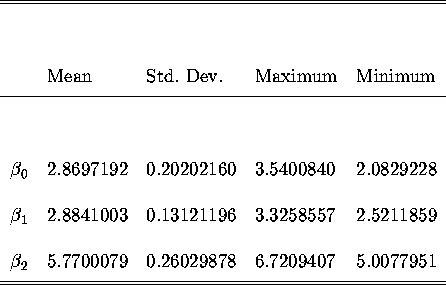
Summary Statistics of OLS estimates from the Montel Carlo experiment are:

Comparing with the true parameter values, it's clear that we are getting biased and inconsistent estimates.

Question 3

Please refer to the sample GAUSS program for this question.

The assumptions made include and , and that are i.i.d. Under these assumptions, OLS estimates will have a lot of nice properties, including BLUE, consistency and asymptotic normality. This is also a simple start to make estimation easier. But you should bear in mind when you conduct serious research in the future that many of these assumptions are far too restrictive.

In my estimation, the dependent variable, a measure of earning power, is given by the hourly wage of the individual (earnings divided by total number of hours worked). Explanatory variables include:

1. a constant term
2. educ: number of years of education
3. ba: a dummy variable that equals 1 if respondent has received a college degree
4. male: a dummy variable that equals 1 if respondent is male
5. white: a dummy variable that equals 1 if respondent is white
6. married: a dummy variable that equals 1 if respondent is married
7. age: age of respondent

For each variable, I have screened out invalid response. Also, I have screened out respondents who work less than 1600 hours, as I believe these are part-time workers and the wage determination of full and part time may be very different. As one of you observed, there are some outliers who earn a whole lot than others. I eliminate the observation of the individual with the highest hourly wage (that person earned an hourly wage of $3400, while the mean hourly wage is just $20). Such outliers can imply coding error. Even if it is coded correctly, the error is too noisy to be added in.

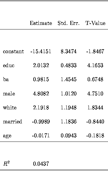
The results of the OLS regression are as follows:

The education variables, educ and ba, are significant and of the sign we expect. More education brings higher earning power. The other education variable, voctrn, is not included because of missing values. Voctrn it is not a variable as good as the other two due to the fact that vocational training are likely to be received for people in occupations with low income, so the variable can be endogenous, and the positive effect of traning on income is blurred. The result also shows that male and white receive significantly higher earnings than female and non-white. Married people have lower earnings, but not very significant. Finally, age is insignificantly negative. Probably age is not a good variable to include. On the one hand, older people may have more work experience, hence higher earnings. But older people's productivity may be declining, bringing lower earnings. The overall effect is really ambiguous.

The regression model explains only of the variation in earning power. This can signal a lot of missing variables, like occupation, skills, and quality of education. Omitted variables can lead to biased and inconsistent estimates. The bad fit can also signal the fact that the model is not linear. Again, this can lead to biasedness and inconsistency. For more careful research, we should proceed to improve our linear regression model, and to collect more relevant explanatory variables.

• About this document ...